Adaptive Gradient Clipping

Gradient Clipping to remove batchnorm layers.

Adaptive Gradient Clipping introduced in the paper “High-Performance Large-Scale Image Recognition Without Normalization” from DeepMind by Brock et al. (2021)

From GC to Adaptive GC

Pascanu, Mikolov, and Bengio (2013) first introduced the gradient clipping technique: for model parameters \(\theta\) and loss function \(L\), the gradient for a particular layer/group of weights(\(l\)) \(G^l\) is \(G^l = \frac{\partial L}{\partial \theta^l}\). Now, Gradient clipping scales down the gradient based on it’s norm.

\[ G^l \rightarrow \begin{cases} \lambda \frac{G^l}{\vert\vert G^l\vert\vert},& \text{if } \vert\vert G^l\vert\vert > \lambda\\ G^l, & \text{otherwise} \end{cases} \]

Here, the gradient clipping is performed independent of the weights it affects, i.e it only dependent on \(G\). Brock et al. (2021) suggests Adaptive Gradient Clipping: if by modifying the gradient clipping condition by introducing the Frobenius norm of the weights(\(W^l\)) the gradient is updating and the gradient \(G^l\) for each block \(i\) in \(\theta\) parameters:

\[ G_i^l \rightarrow \begin{cases} \lambda\frac{\vert\vert W_i^l\vert\vert_F^*}{\vert\vert G_i^l\vert\vert_F},& \text{if } \frac{\vert\vert G_i^l\vert\vert_F}{\vert\vert W_i^l\vert\vert_F^*} > \lambda \\ G_i^l,& \text{otherwise } \end{cases} \\ where \hspace{1mm} {\vert\vert W_i^l\vert\vert_F^*} = max({\vert\vert W_i^l\vert\vert_F^*}, \epsilon) \]

Notice that the condition that regulates the gradient norm depends on the norm with respect to the block of weights its being used to update. Hence, if the gradient is too big for the weights or the weights are too small for the gradient, this clipping strategy suggests to scale the gradient down. This property makes the clipping adaptive.

You might find yourself wondering now, “This is cool, but this doesn’t solve the normalization of features that BatchNorm provides, so where’s that?”. Here, the second trick adapted from a previous paper by the first author Brock, De, and Smith (2021) that introduces - Weight Standardization and Activation scaling

\[ \text{Weight standardization: } \hat W_{ij}= \frac{W_{ij} - \mu_i}{\sqrt N \sigma_i} \]

where \((mean)\mu = (1/N) \sum_j W_{ij}\), \((variance) \sigma_i^2 = (1/N)\sum_j (W_{ij} - \mu)^2\) and \(N\) is fan-in i.e number of input units. In activation scaling, \(\gamma\) is used to scale the activation outputs, where \(\gamma = \sqrt{2/(1 - (1/\pi))}\) for ReLUs.

You can find this code in class WSConv2d here. Notice that the weight that is being used to convoluted is being called in every forward pass. The weight is now reshaped to a 2D tensor - output_channels * (input_channels * (kernel ** 2)) - where i is output_channels and rest is j. Hence, the number of inputs to this is input_channels * (kernel ** 2) i.e. the fan-in parameter. PyTorch’s ONNX export didn’t support mean_var as of that release, hence the mean and variance are calculated separately.

Weighted Residual Connections

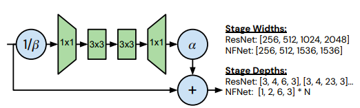
Residual connections have traditionally been \(h_{i+1} = h_i + f_i(h_i)\), where \(h_i\) is input to the residual block \(f_i\). In the NF family of networks, it is modified to \(h_{i+1} = h_i + \alpha f_i(h_i/\beta_i)\). Intuitively, this translates to \(\alpha\) scaling the residual block activations to increase variance and \(\beta\) to scale down the input of the function inside the residual block, as opposed to setting it as identity. \(\alpha\) is set to 0.2 and \(\beta\) is predicted as \(\beta=\sqrt{Variance(h_i)}\).

Batch size intricacies

As Yannic Kilcher explains, there is an implicit dependence on the batch size in AGC, while BatchNorm has an explicit dependence on the batch size. However, the paper doesn’t clearly mention how disentangling the above components effect the accuracy, etc.

Conclusion

To summarize the contributions, Weight standardization and Activation Scaling in combination control the mean-shift at initialization that BatchNorm provides. The Adaptive Gradient Clipping helps prevent the shift by making sure the parameters don’t significantly grow.

These techniques are used in the NAS pipeline to discover the family of architectures the authors term as NFNets. Hence, all of the above techniques combined eliminates the mean-shift - the central role of BatchNorm. This technique scales well with large training batch sizes. The PyTorch code is available on GitHub

https://github.com/vballoli/nfnets-pytorch

Prospective areas

There are interesting future avenues using these tricks. Specifically, in Meta Learning for classification where BatchNorm plays a significant role and how the pre-training on these gradients effect and translate to task-specific adaptation.